Bioinformatics open source interoperability Hackathon at the Broad Institute

Interoperability Hackathon

On April 7th and 8th, a group of biologists and programmers gathered at the Broad Institute to work on improving interoperability of open-source bioinformatics tools. Organized by the Open Bioinformatics Foundation and GenomeSpace team, this was part of the lead up to the Bioinformatics Open Source Conference (BOSC) in July in Berlin. The event is part of an ongoing series of coding sessions (Codefests or Hackathons) organized by the open bioinformatics community, which give programmers who typically work together remotely a chance to code and discuss in the same place for two days. These have been successful in both producing new code and in building connections which help sustain development of these community projects.

Goals and outcomes

One major challenge in analyzing biological data is interfacing multiple bioinformatics tools. Tools often work independently, and where general architectures like plugins or API exist they are often project specific. This results in isolated islands of data exchange, but transferring data or resources between tools requires work that is often rate-limiting or insurmountable.

Our goal at the hackathon was to provide simple APIs and implementations that help facilitate transfers between multiple islands of functionality. GenomeSpace does this by providing a central hub and API to push and pull from tools. We wanted to generalize this to support multiple tools, and build client implementations that demonstrate this in practice. The long term goal is to encourage tool developers to provide server side APIs compatible with the more general library, making extension of the connector toolkit easier. For developers, the client API would allow them to easily transfer files between multiple tools without needing to learn and implement the specific transfer APIs of each tool.

We called this high level client library Genome Connector (gcon, for short) and took a practical approach by implementing client libraries that provide a common interface to multiple tools: GenomeSpace, Galaxy, BaseSpace, 23andMe and general key-value stores through jClouds. To identify a reasonable amount of work for two days, we focused on file transfer: authentication, finding files, getting and putting files to remote analysis platforms. In addition we defined some critical components for doing biological work:

• File metadata: We need to be able to store arbitrary key/value on objects to assign essential biological information necessary to interpret it, like organisms and genome build. In addition, metadata allows provenance and tracking of files by enabling annotation of files with history and processing steps.
• Filesets: Large biological files have secondary files with indexes, allowing indexed retrieval of data (for example: read bam and bai, variant vcf and idx, tabix gz and tbi). To avoid expensive reindexing, we want to group and transfer these together.

We also identified other useful extensions that would help improve interoperability and facilitate building connected tools, like providing Publish/subscribe hooks to avoid having to poll servers for updates, and smarter approaches to sending data to avoid duplication and unnecessary transfer of data.

The output of our discussion and coding are common Genome Connector implementations in multiple languages. GitHub repositories are available for in-progress Java, Python and Clojure implementations. These wrap multiple diverse tools and expose them through a common top level API, allowing developers to push and pull data from multiple tools.

I’m immensely grateful to the incredible participants who generously donated their time and expertise to help with these projects. For anyone interested we also have detailed documentation on discussions during the hackathon.

Bioinformatics Open Source Conference

If you’re a bioinformatics programmers interested in open source coding and helping answer biological questions by improving usability and connectivity of tools, you’re welcome to join the OpenBio and BOSC communities. We’ve created a biological interoperability mailing list for additional discussion. The next BOSC conference is July 19th and 20th in Berlin, Germany as part of the ISMB conference. There will also be another two day Codefest proceeding BOSC on July 17th and 18th. Abstracts for talks at BOSC are due this Friday, April 12th. Looking forward to seeing everyone at future BOSC and coding events.

The influence of reduced resolution quality scores on alignment and variant calling

BAM file size reduction and quality score binning

We have a large upcoming whole genome sequencing project with Illumina, and they approached us about delivering BAM files with reduced resolution base quality scores. They have a white paper describing the approach, which involves binning scores to reduce resolution. This reduces the number of scores describing the quality of a base from 40 down to 8.

The advantage of this approach is a significant reduction in file size. BAM files use BGZF compression, and the underlying gzip DEFLATE algorithm compresses based on shared text regions. Reducing the number of quality values increases shared blocks and improves compression. This reduces BAM file sizes by 25-35%: an exome BAM file reduced from 5.7Gb to 3.7Gb after quality binning.

The potential downside is that the reduction in quality resolution may impact alignment and variant calling approaches that rely on base quality scores. To assess this, I implemented quality score binning as part of the bcbio-nextgen analysis pipeline using the CRAM toolkit and ran alignment, recalibration, realignment and variant calling on:

• The original unbinned 40-resolution base quality BAM from an NA12878 exome.
• The BAM binned into 8-resolution base qualities before alignment.
• The BAM binned into 8-resolution base qualities before alignment and binned again following base quality score recalibration.

A comparison of alignment and variant calls from the three approaches indicates that binning has nearly no impact on alignment and a small impact on variant calls, primarily in low depth regions.

Alignment differences

We aligned 100bp paired end reads with Novoalign, a quality aware aligner. Comparison of mapped reads showed nearly no impact on total mapped reads. The plot below shows a generic delta of changes in mapped reads across the 22 autosomes alongside the increase in unmapped pairs. Out of 73 million total reads, the changes account for ~0.003% of the total reads. There also did not appear to be any worrisome patterns of loss for specific chromosomes. Overall, there is a minimal impact of quality score binning on the ability to align the reads.

Variant call differences

We called variants using the GATK Unified Genotyper following the best practice recommendations for exomes and then compared calls from original and binned quality scores. Both approaches for binning — pre-binning, and pre-binning plus post-quality recalibration binning — showed similar levels of concordance to non-binned quality scores: 99.81 and 99.78, respectively. Since the additional binning after recalibration provides a smaller prepared BAM file for storage and has a similar impact to pre-binning only, we used this for additional analysis of discordant variants.

The table below shows the discordant differences between the 40 quality score resolution and binned, 8 quality score resolution BAMs. 40 quality discordant variants are those called with full quality score resolution but not called, or called differently, after binning to 8 quality score resolution. Conversely, the 8-quality discordants are those called uniquely after quality binning:

Overall genotype concordance	99.78
concordant: total	117887
concordant: SNPs	109144
concordant: indels	8743
40-quality discordant: total	821
40-quality discordant: SNPs	759
40-quality discordant: indels	62
8-quality discordant: total	1289
8-quality discordant: SNPs	1240
8-quality discordant: indels	49
het/hom discordant	259

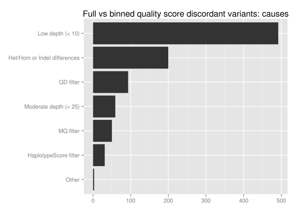
We investigated the discordant variants further since 1.5% of the total variant calls change as a result of binning, Of the 1851 unique discordant variants, approximately half (928) fall into reproducible variants identified by looking at ensemble combinations of replicates. Of these potentially problematic discordant variants more than half are in low coverage regions with less than 10 reads:

The major influence of quality score binning is resolution of variants in low coverage regions. This manifests as differences in heterozygote and homozygote calling, indel representation and filtering differences related to quality and mappability. To assess the potential impact, we looked at the loss in callable bases on a 30x whole genome sequence when moving from a minimum of 5 reads to a minimum of 10, using GATK’s CallableLoci tool. Regions with read coverage of 5 to 9 make up 4.7 million genome positions, 0.17% of the total callable bases.

	5 read minimum	10 read minimum
Callable bases	2,775,871,235	2,771,109,000
Percent callable	96.90%	96.73%
Low coverage	17,641,980	22,404,215
No coverage/ poor mapping	71,272,008	71,272,008

In conclusion, quality score binning provides a useful reduction in input file sizes with minimal impact on alignment. For variant calling, use additional caution in low coverage regions with less than 10 supporting reads. Given the rapid increases in read throughput that are driving the need for file size reduction, quality score binning is a worthwhile tradeoff for high-coverage recalling work.

An automated ensemble method for combining and evaluating genomic variants from multiple callers

Overview

A key goal of the Archon Genomics X Prize infrastructure is development of a set of highly accurate reference genome variants. I’ve described our work preparing these reference genomes, and specifically defined the challenges behind merging genomic variant calls from multiple technologies and calling methods. Comparing calls from two different calling methods, for example GATK and samtools mpileup, produces a large number of differing variants which need reconciliation. Taking the overlapping subset from multiple callers is too conservative and will miss real variations, while including all calls is too liberal and introduces false positives.

Here I’ll describe a fully automated approach for preparing an accurate set of combined variant calls. Ensemble machine learning methods are a powerful way to incorporate inputs from multiple models. We use a heuristic and support vector machine (SVM) algorithm to consolidate variants, producing a final set of calls with better sensitivity and specificity than current best practice methods. The approach is open source, fully automated and generalizable to both human diploid sequencing as well as X Prize haploid reference fosmids.

We use a pair of replicates from EdgeBio’s clinical exome sequencing pipeline to prepare ensemble variant calls in the widely studied HapMap NA12878 genome. Compared to variants from a single calling method, the ensemble method produced more concordant variants when comparing the replicates, with fewer discordants. The finalized ensemble calls also provide a useful method to compare strengths and weaknesses of individual calling methods. The implementation is freely available and I’ll discuss how to get it running on your data so you can use, critique and extend the methods. This work is a collaboration between Harvard School of Public Health, EdgeBio and NIST.

Comparison materials and algorithm

A difficult aspect of evaluating variant calling methods is establishing a reference set of calls. For X Prize we use three established methods, each of which comes with tradeoffs. Metrics like transition/transversion ratios or dbSNP overlap provide a global picture of calling but are not fine grained enough to distinguish improvements over best practices. Sanger validation restricts you to a manageable subset of calls. Comparisons against public resources like 1000 genomes bias results towards technologies and callers used in preparing those variant callsets.

Here we employ a fourth method by comparing replicates from EdgeBio’s clinical exome sequencing pipeline. These are NA12878 samples independently prepared using Nimblegen’s version 3.0 kit and sequenced on an Illumina HiSeq. By comparing the replicates in regions with 4 or more reads in both samples, we identify the ability of variant calling algorithms to call identical variations with differing coverage and error profiles.

We aligned reads with novoalign and performed deduplication, base recalibration and realignment using GATK best practices. With these prepared reads, we called variants with five approaches:

• GATK UnifiedGenotyper – Bayesian approach to call SNPs and indels, treating each position independently.
• GATK HaplotypeCaller – Performs local de-novo assembly to call SNPs and indels on individual haplotypes.
• FreeBayes – Bayesian calling approach that handles simultaneous SNPs and indel calling via assessment of regional haplotypes.
• samtools mpileup – Uses an approach similar to GATK’s UnifiedGenotyper for SNP and indel calling.
• VarScan – Calls variants using a heuristic/statistic approach eliminating common sources of bias.

We took a combined heuristic and machine learning approach to consolidate these five sets of variant calls into a final ensemble callset. The first step is to prepare the union of all variant calls from the input callers, identifying calling methods that support each variant. Secondly, we annotate each variant with metrics including strand bias, allele balance, regional sequence entropy, position of calls within reads, regional base quality and overall genotype likelihoods. We then filter this prepared set of all possible variants to produce a final set of trusted calls.

The first filtering step is to heuristically identify trusted variants based on the number of callers supporting them. This configurable parameter allow you to make an initial conservative cutoff for including variants in the final calls: I trust variants supported by N or more callers.

For the remaining calls that fall below the trusted support cutoff, we distinguish true and false positives using a support vector machine (SVM). The annotated metrics described above are the input parameters and we prepare true and false positives for the classifier using a multi-step process:

• Use variants found in all callers as the true positive set, and variants found in a single caller as false positives. Use these training variants to identify an initial set of below-cutoff variants to include and exclude.
• With this initial set of below-cutoff true/false variants, re-train multiple classifiers stratified based on variant characteristics: variant type (indels vs SNPs), zygosity (heterozygous vs homozygous) and regional sequence complexity.
• Use these final classifiers to identify included and excluded variants falling below the trusted calling support cutoff.

The final set of calls includes the trusted variants and those that pass the SVM filtering. An input configuration file for variant preparation and assessment allows adjustment of the trusted threshold as well as defining which metrics to use for building the SVM classifiers.

Ensemble calling improvements

We assess calling sensitivity and specificity by comparing concordant and discordant variant calls between the replicates. To provide a consistent method to measure both SNP and indel correctness, we use the positive predictive value as the percentage of concordant calls between duplicates (concordant variants / (concordant variants + discordant variants)). This is different than the overall concordance rate, which also includes non-variant regions where both replicates do not call a variation. As a result these percentages will be lower if you expect the 99% values that result when including reference calls. The advantage of this metric is that it’s easily interpreted as the percentage of concordant called variants. It also allows individual comparisons of SNPs and indels, since the overall number of indels are low compared to the total bases considered. GATK’s VariantEval documentation has a nice discussion of alternative metrics to genotype concordance.

As a baseline we used calls from GATK’s UnifiedGenotyper to represent a current best practice approach. GATK calls 117079 SNPs, 86.6% of which are concordant. It also calls 14966 indels, with 64.6% concordant. Here are the full concordant and discordant numbers, broken down by variant type and replicate:

concordant: total	111159
concordant: SNPs	101495
concordant: indels	9664
rep1 discordant: total	9857
rep1 discordant: SNPs	7514
rep1 discordant: indels	2343
rep2 discordant: total	11029
rep2 discordant: SNPs	8070
rep2 discordant: indels	2959
het/hom discordant	4181

Our ensemble method produces improvements in both total concordant variants detected and the ratio of concordant to discordants. For SNPs, the ensemble calls add 5345 additional variants to a total of 122424, with an increase in concordance to 87.4%. For indels the major improvement is in removal of discordants: We identify 14184 indels with 67.2% concordant. Here is the equivalent table for the ensemble method:

concordant: total	116608
concordant: SNPs	107063
concordant: indels	9545
rep1 discordant: total	9555
rep1 discordant: SNPs	7581
rep1 discordant: indels	1974
rep2 discordant: total	10445
rep2 discordant: SNPs	7780
rep2 discordant: indels	2665
het/hom discordant	3975

For scientists who have worked to increase sensitivity and specificity of individual variant callers, it’s exciting to be able to improve both simultaneously. As mentioned above, you can also tune the method to increase specificity or sensitivity by adjusting the support needed for including trusted variants.

The final ensemble callsets from both replicates are available as VCF files from GenomeSpace in the xprize/NA12878-exome-v_03 folder:

• NA12878 exome ensemble calls, replicate 1 – Variants (VCF), Callable regions (BED)
• NA12878 exome ensemble calls, replicate 2 – Variants (VCF), Callable regions (BED)

Comparison of calling methods

Calling the same samples with multiple callers allows direct comparisons between calling methods. The advantage of producing an accurate final set of ensemble calls is that this provides a baseline to evaluate the strengths and weaknesses of different calling methods. The figure below compares concordant, missing variants and additional variants called by each of the 5 methods in comparison with the consolidated ensemble calls:

• GATK UnifiedGenotyper provides the best SNP calling, followed closely by samtools mpileup.
• For indel calling, the GATK HaplotypeCaller produces the most concordant calls followed by UnifiedGenotyper and FreeBayes. UnifiedGenotyper does good as well, but is conservative and has the fewest additional indels. FreeBayes and GATK HaplotypeCaller both provide resolution of individual haplotypes which helps in regions with heterozygous indels or closely spaced SNPs and indels.
• If you want to use a single variant caller, GATK UnifiedGenotyper does the best overall job.
• If you wanted to choose free open-source tools for calling, I would recommend samtools for SNP calling and FreeBayes for indel calling.

Variant calling methods with recommendations for both calling and filtering provide the best out of the box performance. An advantage of GATK and samtools is they provide calling, variant quality metrics, and filtering. On the other side, FreeBayes is a good example of a powerful tool that takes some time to learn to filter optimally. One potential source of bias in producing the individual calls is that I personally have more experience with GATK tools so may have room to improve with the other callers.

Availability and usage

Combining multiple calling approaches improves both sensitivity and specificity of the final set of variants. The downside is the need to run and coordinate calls from all of the different callers. To mitigate this, we developed an automated pipeline that ties together multiple open-source tools using two custom components:

• bcbio-nextgen – A Python framework to run a full sequencing analysis pipeline from input fastq files to consolidated ensemble variant calls. It supports multiple aligners and variant callers, and enables distributed work over multiple cores on a large machine or multiple machines in a cluster environment.
• bcbio.variation – A Clojure toolkit build on top of GATK’s variant API that provides ensemble call preparation as well as more general functionality for normalizing and comparing variants produced by multiple callers.

bcbio-nextgen has a script, built on functionality in the CloudBioLinux project, that automates installation of associated variant callers and data dependencies:

wget https://raw.github.com/chapmanb/bcbio-nextgen/master/scripts/bcbio_nextgen_install.py
python bcbio_nextgen_install.py install_directory data_directory

With the dependencies installed, you describe the input files and analysis with a YAML formatted input file. The NA12878 ensemble configuration file used for this analysis provides a useful starting point. Run the analysis, distributed on multiple cores, with:

bcbio_nextgen.py bcbio_system.yaml ensemble_sample.yaml -n 8

The bcbio-nextgen documentation provides additional details about configuration inputs and distributed processing. The framework generally handles the automation and processing involved with high throughput sequencing analysis.

EdgeBio kindly made the NA12878 datasets used in this analysis publicly available:

• NA12878-NGv3-LAB1360-A (replicate 1)
• NA12878-NGv3-LAB1363-A (replicate 2)

I welcome feedback on the approach, data or tools and am actively working to extend this and make it easier to use. As re-sequencing becomes increasingly important for human health applications it is critical that we develop open, shared best-practice workflows to handle the data processing. This allows us to focus back on the fun and difficult work of understanding the biology.

Genomics X Prize public phase update: variant classification and de novo calling

Background

Last month I described our work at HSPH and EdgeBio preparing reference genomes for the Archon Genomics X Prize public phase, detailing methods used in the first version of our NA19239 variant calls. We’ve been steadily improving the calling approaches, and released version 0.2 on the X Prize validation website and GenomeSpace. Here I’ll describe the improvements we’ve made over the last month, focusing on two specific areas:

• De novo calling: Zam Iqbal suggested using his cortex_var de novo variant caller in addition to the current GATK, FreeBayes and samtools callers. With his help, we’ve included these calls in this release, and provide comparisons between de novo and alignment based methods.
• Improved variant classification: Consolidating variant calls from multiple callers involves making tough choices about when to include or exclude variants. I’ll describe the details of selecting metrics for use in SVM classification and filtering of variants.

Our goal is to iteratively improve our calling and variant preparation to create the best possible set of reference calls. I’d be happy to talk more with anyone working on similar problems or with insight into useful ways to improve our current callsets. We have a Get Satisfaction site for discussion and feedback, and have offered a $2500 prize for helpful comments.

As a reminder, all of the code and data used here is freely available:

• The variant analysis infrastructure, built on top of GATK, automates genome preparation, normalization and comparison. It provides a full pipeline, driven by simple configuration files, for consolidating multiple variant calls.
• The combined variant calls, including training data and potential true and false positives, are available from GenomeSpace: Public/chapmanb/xprize/NA19239-v0_2.
• The individual variant calls for each technology and calling method are also available from GenomeSpace: Public/EdgeBio/PublicData/Release1.

de novo variant calling with cortex_var

de novo variant calling performs reference-free assembly of either local or global genome regions, then subsequently uses these assemblies to call variants relative to a known reference. The advantage is that assemblies can avoid errors associated with mapping to the reference, helping resolve large variations as well as small variations near problem alignments or low complexity regions.

Hybrid approaches that use localized de novo assembly in variant regions help mitigate the extensive computational requirements associated with whole-genome assembly. Complete Genomics variant calling and GATK 2.0’s Haplotype Caller both provide pipelines for hybrid de novo assembly in variant detection. The fermi and SGA assemblers are also used in variant calling, although the paths from assembly to variants are not as automated.

Thanks to Zam’s generous assistance, we used cortex_var for localized de novo assembly and variant calling within individual fosmid boundaries. As a result, CloudBioLinux now contains automated build instructions for cortex_var , handling binary builds for multiple k-mer and color combinations. An automated cortex_var pipeline, part of the bcbio-nextgen toolkit, runs the processing workflow:

• Start with reads aligned to fosmid regions using novoalign.
• For each fosmid region, extract all mapped reads along with a local reference genome for variant calling.
• de novo assemble all reads in the fosmid region and call variants against the local reference genome using cortex_var’s Bubble Caller.
• Remap regional variant coordinates back to the full genome.
• Combine all regional calls into the final set of cortex_var calls.

Directly comparing GATK and cortex_var calls shows similar levels of concordance and discordance as the GATK/samtools comparison from the last post:

concordant: total	153787
concordant: SNPs	130913
concordant: indels	22874
GATK discordant: total	20495
GATK discordant: SNPs	6522
GATK discordant: indels	13973
cortex_var discordant: total	26790
cortex_var discordant: SNPs	21342
cortex_var discordant: indels	5448

11% of the GATK calls and 14% of the cortex_var calls are discordant. The one area where cortex_var does especially well is on indels: 19% of the cortex_var indels do not agree with GATK, in comparison with 37% of the GATK calls and 25% of the samtools calls. The current downside to this is SNP calling, where cortex_var has 3 times more discordant calls than GATK.

Selection of classification metrics

Overlapping variant calls from different calling methods (GATK, FreeBayes, samtools and cortex_var) and sequencing technologies (Illumina, SOLiD and IonTorrent) produces 170,286 potential calls in the fosmid regions. 58% (99,227) of these are present in all callers and technologies, so we need to do better than the intersection in creating a consolidated callset.

As detailed in the previous post, we filter the full set in two ways. The first is to keep trusted variants based on their presence in a defined number of technologies or callers. We currently have an inclusive set of criteria: keep variants present in either 4 out of the 7 callsets, 2 distinct technologies, or 3 distinct callers. This creates a trusted set containing 95% (162,202) of the variants. Longer term the goal is to reduce the trusted count and rely on automated filtering approaches based on input metrics.

This second automated filtering step uses a support vector machine (SVM) to evaluate the remaining variants. We train the SVM on potential true positives from variants that overlap in all callers and technologies, and potential false positives found uniquely in one single caller. The challenge is to find useful metrics associated with these training variants that will help provide discrimination.

In version 0.1 we filtered with a vanilla set of metrics: depth and variant quality score. To identify additional metrics, we used a great variant visualization tool developed by Keming Labs alongside HSPH and EdgeBio. I’ll write up more details about the tool once we have a demonstration website but the code is already available on GitHub.

To remove variants preferentially associated with poorly mapping or misaligned reads, we identified two useful metrics. ReadPosEndDist, written as a GATK annotation by Justin Zook at NIST, identifies variants primarily supported by calls at the ends of reads. Based on visual examination, these associate with difficult to map regions, as identified by Genome Mappability Scores:

Secondly, we identified problematic allele balances that differ from the expected ratios. For haploid fosmid calls, we expect 100% of reads to support variants and 0% to support reference calls (in diploid calls, you also need to handle heterozygotes with 50% expected allele balance). In practice, the distribution of reads can differ due to sequencer and alignment errors. We use a metric that measures deviation from the expected allele balance and associates closely with variant likelihoods:

Improved consolidated calls

To assess the influence of adding de novo calls and additional filtering metrics on the resulting call set, we compare against whole genome Illumina and Complete Genomics calls for NA19239. Previously we’d noticed two major issues during this comparison: a high percentage of discordant indel calls and a technology bias signaled by better concordance with Illumina than Complete.

The comparison between fosmid and Illumina data shows a substantial improvement in the indel bias. Previously 46% of the total indel calls were discordant, indicative of a potential false positive problem. With de novo calls and improved filtering, we’ve lowered this to only 10% of the total calls.

concordant: total	147684
concordant: SNPs	133861
concordant: indels	13823
fosmid discordant: total	7519
fosmid discordant: SNPs	5856
fosmid discordant: indels	1663
Illumina discordant: total	5640
Illumina discordant: SNPs	1843
Illumina discordant: indels	3797

This improvement comes with a decrease in the total number of concordant indel calls, since we moved from 17,816 calls to 13,823. However a large number of these seemed to be Illumina specific since 60% of the previous calls were discordant when compared with Complete Genomics. The new callset reduces this discrepancy and only 22% of the indels are now discordant:

concordant: total	139155
concordant: SNPs	127243
concordant: indels	11912
fosmid discordant: total	15484
fosmid discordant: SNPs	12028
fosmid discordant: indels	3456
Complete Genomics discordant: total	7311
Complete Genomics discordant: SNPs	4972
Complete Genomics discordant: indels	2273

These comparisons provide some nice confirmation that we’re moving in the right direction on filtering. As before, we extract potential false positives and false negatives to continue to refine the calls: potential false positives are those called in the fosmid dataset and in neither of the Illumina or Complete Genomics sets. Potential false negatives are calls that both Illumina and Complete agree on that the fosmid calls lack.

In the new callsets, there are 5,499 (3.5%) potential false positives and 1,422 (0.9%) potential false negatives. We’ve reduced potential false positives in the previous set from 10% with a slight increase in false negatives. These subsets are available along with the full callset on GenomeSpace. We’re also working hard on an NA12878 callset with equivalent approaches and will make that available soon for community feedback.

I hope this discussion, open source code, and dataset release is useful to everyone working on problems of improving variant calling accuracy and filtering. I welcome feedback on calling, consolidation methods, interesting metrics to explore, machine learning or any of the other topics discussed here.

Genomics X Prize public phase: reference genome preparation and comparisons to Illumina and Complete Genomics

Background

The Archon Genomics X Prize, presented by Express Scripts, is a 10 million dollar competition to establish highly accurate clinical grade sequencing and variation detection methods. Our group at Harvard School of Public Health works with the EdgeBio team on developing the infrastructure for the competition: identify variations in the grading genomes and provide software to compare these reference variation sets against a competitor’s list of variations.

The exciting aspect of the Genomics X Prize is that it enables open comparisons between sequencing technologies and variant calling methodologies. Sequencing genomes to the high degree of accuracy sufficient for clinical usage is a difficult, open, problem. Here I’ll present detailed numbers comparing variants called by different sequencing technologies and variant callers.

The public phase of the Genomics X Prize starts today, August 15th. The goal of this six month period is to have an open dialog with everyone working in the sequencing and variant calling communities. We want to refine our methods to provide the most accurate and fair variant calling for the reference genomes. To start the discussion we’ve prepared:

• Variant calls for a HapMap individual: NA19239, a Yoruba male from Ibadan, Nigeria. We sequenced haploid fosmids from NA19239 with two technologies: Illumina and SOLiD; and called variants with three different methods: GATK Unified Genotyper, FreeBayes, and SAMtools mpileup. We combined these calls into a unified final call set, NA19239 version 0.1, that I discuss in detail below.
• Fully documented methods, access to all data files used, and a public scoring site. The X Prize Validation wiki contains detailed information about sequencing, variant calling, validation and scoring. The validationprotocol.org website provides a simple way for anyone to compare their variant calls against the public reference genomes. It encourages submission and analysis in public tools like Galaxy through transparent interoperability with GenomeSpace.
• An automated variant analysis infrastructure built on top of the Broad’s Genome Analysis Toolkit (GATK) that performs comparisons as well as variant unification. This is a generally useful toolkit of functionality to manipulate variants, and we presented an overview at the Bioinformatics Open Source Conference last month. This is an open-source community developed project, and has received great contributions from the Genome in a Bottle Consortium at the National Institute of Standards and Technology.

The goal of this writeup, and the X Prize public phase, is to iterate over calling and unification methods to improve our algorithms and approaches. Rather than promoting or disparaging any particular technology or calling method, we’re instead providing full transparency and a good-faith effort to combining approaches. Our hope is that this will help engage the community, encourage feedback, and result in a unbiased and accurate set of reference genomes for the competition.

Unification of variant calls

For the August 15th public phase kickoff, we prepared a reference data set of NA19239 based on pooled sequencing of haploid fosmid clones. The callable regions of these clones totaled 129,513,026 total bases, covering ~4% of the 3.1 billion bases in the human genome. We use fosmid clones to obtain complete regional haplotype coverage and focus on partial genome coverage to achieve high coverage depth and accuracy for assessed regions.

Version 0.1 of the NA19239 reference set uses variant calls from two technologies: Illumina and SOLiD; and three callers: GATK’s Unified Genotyper, FreeBayes and SAMtools. To move from these data to a unified call set we:

• Align to GRCh37 reference genome with Novoalign.
• Perform post-processing and indel realignment with GATK’s IndelRealigner.
• Perform variant calling with GATK’s UnifiedGenotyper, FreeBayes and samtools mpileup.
• Do pairwise comparisons between all technology/caller approaches.
• Generate the union of all possible calls and merge with initial GATK calls, recalling any no-call positions at expected sites.
• Use validation information on variants found in multiple technologies, plus metrics associated with common variants, to filter the full call set to a final set of trusted calls.

The challenging decisions begin when merging and filtering the final call set. This requires careful bookkeeping and variant representation to ensure identical variants are directly comparable, followed by setting cutoffs for variant inclusion.

Comparison details

The details of variant comparisons introduce an additional layer of complexity during assessment. The approach we’ve taken is create a normalized set of variants so all comparison differences are due to actual call differences rather than variant representation. We split multiple nucleotide polymorphisms into individual calls, split complex indel-variant combinations, and left-align remaining variants.

For haploid/diploid comparisons, we establish haplotype blocks for the diploid sequence based on phasing provided in the input variant file, and then compare the best matching haplotype to our fosmid reference. Single nucleotide polymorphisms and indels less than 30bp require exact machines between two comparison genomes. Larger indels and structural variations receive more flexible matching with confidence intervals around start and end coordinates.

The goal of the normalized, compared variants is to reflect real underlying differences in calling approaches relative to how well we can currently resolve variation endpoints.

Comparisons between variation callers

For a concrete example of two different variant calling approaches, below is a table comparing GATK variants against samtools calls for the NA19239 sample, using identically aligned and post-processed BAMs:

concordant: total	160851
concordant: SNPs	136146
concordant: indels	24705
GATK discordant: total	13925
GATK discordant: SNPs	1315
GATK discordant: indels	12610
samtools discordant: total	25368
samtools discordant: SNPs	17247
samtools discordant: indels	8121

The number of discordant variant calls is high, making up 8% of the GATK calls and 14% of the samtools calls, and samtools calls almost 16,000 additional SNPs compared to GATK. As a result, a large percentage of variants require making hard decisions: are those additional calls interesting, real variants in samtools and false negatives in the GATK calls? Or conversely, are they false positives in samtools that GATK correctly excludes?

Comparisons between sequencing technologies

There is a similar level of discrepancy when comparing variant calls between Illumina and SOLiD sequencing. Below is a comparison between GATK Unified genotyper calls on the two technologies:

concordant: total	135263
concordant: SNPs	122267
concordant: indels	12996
Illumina discordant: total	39491
Illumina discordant: unique	7079
Illumina discordant: SNPs	15188
Illumina discordant: indels	24303
SOLiD discordant: total	16022
SOLiD discordant: unique	3800
SOLiD discordant: SNPs	3908
SOLiD discordant: indels	12114

Unique coverage explains some differences: 4% of the Illumina variants (7079) and 2.5% (3800) of the SOLiD variants were uniquely covered by the technologies. However, the remaining variant discordant calls are on the order of those seen in the technology comparisons. Adding to the complexity, we find only 84% of the total concordant variants compared to the Illumina only GATK/samtools comparison.

Unified call set

The level of discrepancy between calling methods and sequencing approaches introduces complexity in the preparation of the final call set: How much evidence does a variant need for inclusion? Can single calls be true positives if supported by high confidence values? This will require extensive refinement throughout the public phase. For the initial version 0.1 release of NA19239, we took the following high level approach to filtering:

• Retain variants found in 4 out of 6 calling/technology methods (including genotyping data).
• Retain variants identified across multiple technologies.
• Retain variants found in both more stringent (GATK) and more lenient (FreeBayes, samtools) callers.
• Assess remaining variants using a Support Vector Machine with quality score, read depth and variant distance from read ends metrics, training the classifier on likely true and false positives from the pairwise overlap comparisons.

The result is a unified call set of 171,009 variants derived from all technologies and callers, that we’re releasing as NA19239 version 0.1.

Comparisons with whole genome datasets

To assess the quality of the unified call set, we compared to two public genomes:

• Complete Genomics’s NA19239 variants from their public whole genome datasets,
• An Illumina whole genome dataset for NA19239 at 30x coverage.

This provides us with three independent call sets to assess variability between approaches. To provide a baseline, here is the comparison of the Illumina and Complete Genomics calls in our assessment regions:

Overall genotype concordance	98.47
concordant: total	205868
concordant: SNPs	186365
concordant: indels	19503
Illumina discordant: total	31267
Illumina discordant: SNPs	19334
Illumina discordant: indels	11933
Complete Genomics discordant: total	15174
Complete Genomics discordant: SNPs	9586
Complete Genomics discordant: indels	5510

We see familiar discordance rates: 13% of the Illumina calls and 7% of the Complete Genomics calls differ. Since it’s diploid versus diploid, this comparison includes all heterozygous variant matches. As a result the numbers in this comparison will be higher, but it is a good order of magnitude approximation for looking at our fosmid reference set versus each individual technology.

Illumina

The comparison against the Illumina whole genome variant calls contains 12% discordant calls in our fosmid reference set, with 79% of those being indel differences. Indels are notoriously more difficult to identify and assess, so this will be an area of increased focus as we move forward:

concordant: total	150420
concordant: SNPs	132604
concordant: indels	17816
fosmid discordant: total	19624
fosmid discordant: SNPs	4165
fosmid discordant: indels	15459
Illumina discordant: total	5475
Illumina discordant: SNPs	2952
Illumina discordant: indels	2523

Complete Genomics

The Complete Genomics comparison has 17% discordant calls including 2x more discordant SNP calls. This highlights another key area of call set refinement: identifying and correcting for technology specific calls.

concordant: total	139559
concordant: SNPs	126296
concordant: indels	13263
fosmid discordant: total	29883
fosmid discordant: SNPs	10162
fosmid discordant: indels	19721
Complete Genomics discordant: total	7571
Complete Genomics discordant: SNPs	5542
Complete Genomics discordant: indels	1965

Summary

The initial NA19239 public genome for the Genomics X Prize provides unified variant calls based on two sequencing technologies and three calling methods. I’ve delved into a lot of details on our approaches, challenges and goals with the hopes of encouraging suggestions from other researchers working on these problems. We’re especially interested in feedback on these areas of ongoing research:

• Digging deeper into potential false positives and negatives: By combining comparison information between the unified callset and external resources, we can identify 17654 fosmid variants (10%) not found in both the Complete Genomics and Illumina datasets. These require additional in-depth analysis to classify as uniquely identified fosmid calls or potential false positives. Similarly, Illumina and Complete Genomics combine to call 1228 variants (0.7%) that are not in the fosmid call set. These need examination to classify as fosmid false negatives, or false positive calls in the individual technologies.
• Additional public genomes: We’re actively working with teams like the Genome in a Bottle Consortium and Genome Research Consortium to compare with their reference sets and approaches. Our next target public genome is NA12878, used in both of these projects and widely studied.
• Improve variant representation and assessment: The variation software framework works hard to make variant representations as uniform as possible. Indels are especially challenging and we welcome practical examples of regions that need additional standardization.
• Refine approaches to unifying variant calls: What we learn from the additional inspection of discordant variants can help inform improved approaches to filtering. This is a great opportunity to develop generalized, reusable methods for combining variants from multiple approaches.

The call sets used here are available as public data folders on GenomeSpace:

• Public/chapmanb/xprize/NA19239-v0_1 – The combined final call set along with training true/false positives and Illumina/Complete Genomics comparison based potential false positives and negatives.
• Public/EdgeBio/PublicData/Release1 – All of the raw input data, including fastq files, BAM alignments and individual variant calls.

Combined with the open source code and configurations, we hope this will provided interested researchers with all the raw materials needed to reproduce and extend these analyses. Your feedback and suggestions are very welcome.

Extending the GATK for custom variant comparisons using Clojure

The Genome Analysis Toolkit (GATK) is a full-featured library for dealing with next-generation sequencing data. The open-source Java code base, written by the Genome Sequencing and Analysis Group at the Broad Institute, exposes a Map/Reduce framework allowing developers to code custom tools taking advantage of support for: BAM Alignment files through Picard, BED and other interval file formats through Tribble, and variant data in VCF format.

Here I’ll show how to utilize the GATK API from Clojure, a functional, dynamic programming language that targets the Java Virtual Machine. We’ll:

• Write a GATK walker that plots variant quality scores using the Map/Reduce API.
• Create a custom annotation that adds a mean neighboring base quality metric using the GATK VariantAnnotator.
• Use the VariantContext API to parse and access variant information in a VCF file.

The Clojure variation library is freely available and is part of a larger project to provide variant assessment capabilities for the Archon Genomics XPRIZE competition.

Map/Reduce GATK Walker

GATK’s well documented Map/Reduce API eases the development of custom programs for processing BAM and VCF files. The presentation from Eli Lilly is a great introduction to developing your own custom GATK Walkers in Java. Here we’ll follow a similar approach to code these in Clojure.

We’ll start by defining a simple Java base class that extends the base GATK walker and defines an output and input variable. The output is a string specifying the output file to write to, and the input is any type of variant file the GATK accepts. Here we’ll be dealing with VCF input files:

public abstract class BaseVariantWalker extends RodWalker {
  @Output
  public String out;

  @ArgumentCollection
  public StandardVariantContextInputArgumentCollection invrns = new StandardVariantContextInputArgumentCollection();
}

This base class is all the Java we need. We implement the remaining walker in Clojure and will walk through the fully annotated source in sections. To start, we import the base walker we wrote and extend this to generate a Java class, which the GATK will pick up and make available as a command line walker:

(ns bcbio.variation.vcfwalker
  (:import [bcbio.variation BaseVariantWalker])
  (:gen-class
   :name bcbio.variation.vcfwalker.VcfSimpleStatsWalker
   :extends bcbio.variation.BaseVariantWalker))

Since this is a Map/Reduce framework, we first need to implement the map function. GATK passes this function a tracker, used to retrieve the actual variant call values and a context which describes the current location. We use the invrns argument we defined in Java to reference the input VCF file supplied on the commandline. Finally, we extract the quality score from each VariantContext and return those. This map function produces a stream of quality scores from the input VCF file:

(defn -map
  [this tracker ref context]
  (if-not (nil? tracker)
    (for [vc (map from-vc
                    (.getValues tracker (.variants (.invrns this))
                                (.getLocation context)))]
      (-> vc :genotypes first :qual))))

For the reduce part, we take the stream of quality scores and plot a histogram. In the GATK this happens in 3 functions: reduceInit starts the reduction step and creates a list to add the quality scores to, reduce collects all of the quality scores into this list, and onTraversalDone plots a histogram of these scores using the Incanter statistical library:

(defn -reduceInit
  [this]
  [])

(defn -reduce
  [this cur coll]
  (if-not (nil? cur)
    (vec (flatten [coll cur]))
    coll))

(defn -onTraversalDone
  [this result]
  (doto (icharts/histogram result
                           :x-label "Variant quality"
                           :nbins 50)
    (icore/save (.out this) :width 500 :height 400)))

We’ve implemented a full GATK walker in Clojure, taking advantage of existing Clojure plotting libraries. To run this, compile the code into a jarfile and run like a standard GATK tool:

$ lein uberjar
$ java -jar bcbio.variation-0.0.1-SNAPSHOT-standalone.jar -T VcfSimpleStats
  -r test/data/grch37.fa --variant test/data/gatk-calls.vcf --out test.png

which produces a plot of quality score distributions:

Custom GATK Annotation

GATK’s Variant Annotator is a useful way to add metrics information to a file of variants. These metrics allow filtering and prioritization of variants, either by variant quality score recalibration or hard filtering. We can add new annotation metrics by inheriting from GATK Java interfaces. Here we’ll implement Mean Neighboring Base Quality (NBQ), a metric from the Atlas2 variation suite that assesses the quality scores in a region surrounding a variation.

We start walking through the full implementation by again defining a generated Java class that inherits from a GATK interface. In this case, InfoFieldAnnotation:

(ns bcbio.variation.annotate.nbq
  (:import [org.broadinstitute.sting.gatk.walkers.annotator.interfaces.InfoFieldAnnotation]
           [org.broadinstitute.sting.utils.codecs.vcf VCFInfoHeaderLine VCFHeaderLineType])
  (:require [incanter.stats :as istats])
  (:gen-class
   :name bcbio.variation.annotate.nbq.MeanNeighboringBaseQuality
   :extends org.broadinstitute.sting.gatk.walkers.annotator.interfaces.InfoFieldAnnotation))

The annotate function does the work of calculating the mean quality score. We define functions that use the GATK API to:

• Retrieve the pileup at the current position.
• Get the neighbor qualities from a read at a position.
• Combine the qualities for all reads in a pileup.

With these three functions, we can use the Clojure threading macro to cleanly organize the steps of the operation as we retrieve the pileup, get the qualities and calculate the mean:

(defn -annotate
  [_ _ _ _ contexts _]
  (letfn [(get-pileup [context]
            (if (.hasExtendedEventPileup context)
              (.getExtendedEventPileup context)
              (.getBasePileup context)))
          (neighbor-qualities [[offset read]]
            (let [quals (-> read .getBaseQualities vec)]
              (map #(nth quals % nil) (range (- offset flank-bp) (+ offset flank-bp)))))
          (pileup-qualities [pileup]
            (map neighbor-qualities (map vector (.getOffsets pileup) (.getReads pileup))))]
    {"NBQ" (->> contexts
                vals
                (map get-pileup)
                (map pileup-qualities)
                flatten
                (remove nil?)
                istats/mean
                (format "%.2f"))}))

With this in place we can now run this directly using the standard GATK command line arguments. As before, we create a jar file with the new annotator, and then pass the name as a desired annotation when running the VariantAnnotator, producing a VCF file with NBQ annotations:

$ lein uberjar
$ java -jar bcbio.variation-0.0.1-SNAPSHOT-standalone.jar -T VariantAnnotator
   -A MeanNeighboringBaseQuality -R test/data/GRCh37.fa -I test/data/aligned-reads.bam
   --variant test/data/gatk-calls.vcf -o annotated-file.vcf

Access VCF variant information

In addition to extending the GATK through walkers and annotations you can also utilize the extensive API directly, taking advantage of parsers and data structures to handle common file formats. Using Clojure’s Java interoperability, the variantcontext module provides a high level API to parse and extract information from VCF files. To loop through a VCF file and print the location, reference allele and called alleles for each variant we:

• Open a VCF source providing access to the underlying file inside a with-open statement to ensure closing of the resource.
• Parse the VCF source, returning an iterator of VariantContext maps for each variant in the file.
• Extract values from the map: the chromosome, start, reference allele and called alleles for the first genotype.

(use 'bcbio.variation.variantcontext)

(with-open [vcf-source (get-vcf-source "test/data/gatk-calls.vcf")]
  (doseq [vc (parse-vcf vcf-source)]
    (println (:chr vc) (:start vc) (:ref-allele vc)
             (-> vc :genotypes first :alleles)))

This produces:

MT 73 #<Allele G*> [#<Allele A> #<Allele A>]
MT 150 #<Allele T*> [#<Allele C> #<Allele C>]
MT 152 #<Allele T*> [#<Allele C> #<Allele C>]
MT 195 #<Allele C*> [#<Allele T> #<Allele T>]

I hope this tour provides some insight into the powerful tools that can be rapidly built by leveraging the GATK from Clojure. The full library contains a range of additional functionality including normalization of complex MNPs and support for phased haplotype comparisons.

Making next-generation sequencing analysis pipelines easier with BioCloudCentral and Galaxy integration

My previous post described running an automated exome pipeline using CloudBioLinux and CloudMan, and generated incredibly useful feedback. Comments and e-mails pointed out potential points of confusion for new users deploying the process on custom data. I also had the chance to get hands on with researchers running CloudBioLinux and CloudMan during the AWS Genomics Event (talk slides are available).

The culmination of all this feedback are two new development projects from the CloudBioLinux community, aimed at making it easier to run custom analysis pipelines:

• BioCloudCentral — A web service that launches CloudBioLinux and CloudMan clusters on Amazon Web Services hardware. This removes all of the manual steps involved in setting up security groups and launching a CloudBioLinux instance. A user only needs to sign up for an AWS account; BioCloudCentral takes care of everything else.

• A custom Galaxy integrated front-end to next-generation sequencing pipelines. A jQuery UI wizard interface manages the intake of sequences and specification of parameters. It runs an automated backend processing pipeline with the structured input data, uploading results into Galaxy data libraries for additional analysis.

Special thanks are due to Enis Afgan for his help building these tools. He provided his boto expertise to the BioCloudCentral Amazon interaction, and generalized CloudMan to support the additional flexibility and automation on display here.

This post describes using these tools to start a CloudMan instance, create an SGE cluster and run a distributed variant calling analysis, all from the browser. The behind the scene details described earlier are available: the piepline uses a CloudBioLinux image containing a wide variety of bioinformatics software and you can use ssh or an NX graphical client to connect to the instance. This is the unique approach behind CloudBioLinux and CloudMan: they provide an open framework for building automated, easy-to-use workflows.

BioCloudCentral — starting a CloudBioLinux instance

To get started, sign up for an Amazon Web services account. This gives you access to on demand computing where you pay per hour of usage. Once signed up, you will need your Access Key ID and Secret Access Key from the Amazon security credentials page.

With these, navigate to BioCloudCentral and fill out the simple entry form. In addition to your access credentials, enter your choice of a name used to identify the cluster, and your choice of password to access the CloudMan web interface and the cluster itself via ssh or NX.

Clicking submit launches a CloudBioLinux server on Amazon. Be careful, since you are now paying per hour for your machine; remember to shut it down when finished.

Before leaving the monitoring page, you want to download a pre-formatted user-data file; this allows you to later start the same CloudMan instance directly from the Amazon web services console.

CloudMan — managing the cluster

The monitoring page on BioCloudCentral provides links directly to the CloudMan web interface. On the welcome page, start a shared CloudMan instance with this identifier:

cm-b53c6f1223f966914df347687f6fc818/shared/2012-07-23--19-23/

This shared instance contains the custom Galaxy interface we will use, along with FASTQ sequence files for demonstration purposes. CloudMan will start up the filesystem, SGE, PostgreSQL and Galaxy. Once launched, you can use the CloudMan interface to add additional machines to your cluster for processing.

Galaxy pipeline interface — running the analysis

This Galaxy instance is a fork of the main codebase containing a custom pipeline interface in addition to all of the standard Galaxy tools. It provides an intuitive way to select FASTQ files for processing. Login with the demonstration account (user: example@example.com; password: example) and load FASTQ files along with target and bait BED files into your active history. Then work through the pipeline wizard step by step to start an analysis:

The Galaxy interface builds a configuration file describing the parameters and inputs, and submits this to the backend analysis server. This server kicks off processing, distributing the analysis across the SGE cluster. For the test data, processing will take approximately 4 hours on a cluster with a single additional work node (Large instance type).

Galaxy — retrieving and displaying results

The analysis pipeline uploads the finalized results into Galaxy data libraries. For this demonstration, the example user has results from a previous run in the data library so you don’t need to wait for the analysis to finish. This folder contains alignment data in BAM format, coverage information in BigWig format, a VCF file of variant calls, a tab separate file with predicted variant effects, and a PDF file of summary information. After importing these into your active Galaxy history, you can perform additional analysis on the data, including visualization in the UCSC genome browser:

As a reminder, don’t forget to terminate your cluster when finished. You can do this either from the CloudMan web interface or the Amazon console.

Analysis pipeline details and extending this work

The backend analysis pipeline is a freely available set of Python modules included on the CloudBioLinux AMI. The pipeline closely follows current best practice variant detection recommendations from the Broad GATK team:

• FASTQ alignment with BWA; source code
• Base quality score recalibration with GATK: source code
• Local realignment around indels with GATK: source code:
• Variant calling (SNPs and indels) using the GATK Unified Genotyper: source code
• Variant effect estimation with snpEff: source code
• Read coverage visualization with wigToBigWig: source code

The pipeline framework design is general, allowing incorporation of alternative aligners or variant calling algorithms.

We hope that in addition to being directly useful, this framework can fit within the work environments of other developers. The flexible toolkit used is: CloudBioLinux with open source bioinformatics libraries, CloudMan with a managed SGE cluster, Galaxy with a custom pipeline interface, and finally Python to parallelize and manage the processing. We invite you to fork and extend any of the different components. Thank you again to everyone for the amazing feedback on the analysis pipeline and CloudBioLinux.

Parallel approaches in next-generation sequencing analysis pipelines

My last post described a distributed exome analysis pipeline implemented on the CloudBioLinux and CloudMan frameworks. This was a practical introduction to running the pipeline on Amazon resources. Here I’ll describe how the pipeline runs in parallel, specifically diagramming the workflow to identify points of parallelization during lane and sample processing.

Incredible innovation in throughput makes parallel processing critical for next-generation sequencing analysis. When a single Hi-Seq run can produce 192 samples (2 flowcells x 8 lanes per flowcell x 12 barcodes per lane), the analysis steps quickly become limited by the number of processing cores available.

The heterogeneity of architectures utilized by researchers is a major challenge in building re-usable systems. A pipeline needs to support powerful multi-core servers, clusters and virtual cloud-based machines. The approach we took is to scale at the level of individual samples, lanes and pipelines, exploiting the embarassingly parallel nature of the computation. An AMQP messaging queue allows for communication between processes, independent of the system architecture. This flexible approach allows the pipeline to serve as a general framework that can be easily adjusted or expanded to incorporate new algorithms and analysis methods.

Process overview — points for parallel implementations

The first level of parallelization occurs during processing of each fastq lane. We split the file into individualized barcoded components, followed by alignment and BAM processing. The result is a sorted BAM file for each barcoded sub-sample, given a set of input fastq files:

The pipeline merges samples present in barcodes on multiple lanes, producing a single representative BAM file. The next step parallelizes the processing of each alignment file with read quality assessment, preparation for visualization and variant calling:

The variant calling steps utilize The Genome Analysis Toolkit (GATK) from the Broad Institute. It prepares alignments by recalibrating initial quality scores given the aligned sequences and consistently realigning reads around indels. The Unified Genotyper identifies variants from this prepared alignment file, then uses these variants along with known true sites for assigning quality scores and filtering to a final set of calls:

Subsequent steps include assessment of variant effects using snpEff and haplotype phasing of variants in diploid organism analyses.

Messaging approach to parallel execution

The process diagrams illustrate points of parallel execution for each fastq file and sample analysis. Practically, a top level analysis server manages each of the sub-processes. A command line script, a LIMS system or a specialized Galaxy interface start this top level process. RabbitMQ messaging facilitates communication between the analysis controller and processing nodes:

In my previous post, CloudMan manages this entire process. The web interface controls a pre-configured SGE cluster and a custom script starts the job on this cluster. However, the general nature of the pipeline architecture allows this to work equally well on multiple core machines or a heterogeneous set of connected machines.

The CloudMan work demonstrates that clusters, especially on-demand virtual images like those available from Amazon, are be a powerful way to scale analyses. Equally important, it provides an open platform to share these pipelines and encourage re-use. The code for the pipeline is available from the bcbio-nextgen GitHub repository

Distributed exome analysis pipeline with CloudBioLinux and CloudMan

A major challenge in building analysis pipelines for next-generation sequencing data is combining a large number of processing steps in a flexible, scalable manner. Current best-practice software needs to be installed and configured alongside the custom code to chain individual programs together. Scaling to handle increasing throughput requires running that custom code on a wide variety of parallel architectures, from single multicore machines to heterogeneous clusters.

Establishing community resources that meet the challenges of building these pipelines ensures that bioinformatics programmers can share the burden of building large scale systems. Two open-source efforts which aim at providing this type of architecture are:

• CloudBioLinux — A community effort to create shared images filled with bioinformatics software and libraries, using an automated build environment.

• CloudMan — Uses CloudBioLinux as a platform to build a full SGE cluster environment. Written by Enis Afgan and the Galaxy Team, CloudMan is used to provide a ready-to-run, dynamically scalable version of Galaxy on Amazon AWS.

Here we combine CloudBioLinux software with a CloudMan SGE cluster to build a fully automated pipeline for processing high throughput exome sequencing data:

• The underlying analysis software is from CloudBioLinux.
• CloudMan provides an SGE cluster managed via a web front end.
• RabbitMQ is used for communication between cluster nodes.
• An automated pipeline, written in Python, organizes parallel processing across the cluster.

Below are instructions for starting a cluster on Amazon EC2 resources to run an exome sequencing pipeline that processes FASTQ sequencing reads, producing fully annotated variant calls.

Start cluster with CloudBioLinux and CloudMan

Start in the Amazon web console, a convenient front end for managing EC2 servers. The first step is to follow the CloudMan setup instructions to create an Amazon account and set up appropriate security groups and user data. The wiki page contains detailed screencasts. Below is a short screencast showing how to boot your CloudBioLinux specific CloudMan server:

Once this is booted, proceed to the CloudMan web interface on the server and startup an instance from this shared identifier:

cm-b53c6f1223f966914df347687f6fc818/shared/2012-07-23--19-23

This screencast shows all of the details, including starting an additional node on the SGE cluster:

Configure AMQP messaging

Edit: The AMQP messaging steps have now been full automated so the configuration steps in this section are no longer required. Skip down to the ‘Run Analysis’ section to start processing the data immediately.

With your server booted and ready to run, the next step is to configure RabbitMQ messaging to communicate between nodes on your cluster. In the AWS console, find the external and internal hostname of the head machine. Start by opening an ssh connection to the machine with the external hostname:

$ ssh -i your-keypair ubuntu@ec2-50-19-177-134.compute-1.amazonaws.com

Edit the /export/data/galaxy/universe_wsgi.ini configuration file to add the internal hostname. After editing, the AMQP section will look like:

[galaxy_amqp]
host = ip-10-125-10-182.ec2.internal
port = 5672
userid = biouser
password = tester

Finally, add the user and virtual host to the running RabbitMQ server on the master node with 3 commands:

$ sudo rabbitmqctl add_user biouser tester
creating user "biouser" ...
...done.
$ sudo rabbitmqctl add_vhost bionextgen
creating vhost "bionextgen" ...
...done.
$ sudo rabbitmqctl set_permissions -p bionextgen biouser ".*" ".*" ".*"
setting permissions for user "biouser" in vhost "bionextgen" ...
...done.

Run analysis

With messaging in place, we are ready to run the analysis. /export/data contains a ready to run example exome analysis, with FASTQ input files in /export/data/exome_example/fastq and configuration information in /export/data/exome_example/config. Start the fully automated pipeline with a single command:

 $ cd /export/data/work
 $ distributed_nextgen_pipeline.py /export/data/galaxy/post_process.yaml
                                   /export/data/exome_example/fastq
                                   /export/data/exome_example/config/run_info.yaml

distributed_nextgen_pipeline.py starts processing servers on each of the cluster nodes, using SGE for scheduling. Then a top level analysis server runs, splitting the FASTQ data across the nodes at each step of the process:

• Alignment with BWA
• Preparation of merged alignment files with Picard
• Recalibration and realignment with GATK
• Variant calling with GATK
• Assessment of predicted variant effects with snpEff
• Preparation of summary PDFs for each sample with read details from FastQC alongside alignment, hybrid selection and variant calling statistics from Picard

Monitor the running process

The example data is from a human chromosome 22 hybrid selection experiment. While running, you can keep track of the progress in several ways. SGEs qstat command will tell you where the analysis servers are running on the cluster:

$ qstat
ob-ID  prior   name   user  state submit/start at   queue
----------------------------------------------------------------------------------
1 0.55500 nextgen_an ubuntu  r  08/14/2011 18:16:32 all.q@ip-10-125-10-182.ec2.int
2 0.55500 nextgen_an ubuntu  r  08/14/2011 18:16:32 all.q@ip-10-86-254-105.ec2.int
3 0.55500 automated_ ubuntu  r  08/14/2011 18:16:47 all.q@ip-10-125-10-182.ec2.int

Listing files in the working directory will show our progress:

$ cd /export/data/work
$ ls -lh
drwxr-xr-x 2 ubuntu ubuntu 4.0K 2011-08-13 21:09 alignments
-rw-r--r-- 1 ubuntu ubuntu 2.0K 2011-08-13 21:17 automated_initial_analysis.py.o11
drwxr-xr-x 2 ubuntu ubuntu   33 2011-08-13 20:43 log
-rw-r--r-- 1 ubuntu ubuntu  15K 2011-08-13 21:17 nextgen_analysis_server.py.o10
-rw-r--r-- 1 ubuntu ubuntu  15K 2011-08-13 21:17 nextgen_analysis_server.py.o9
drwxr-xr-x 8 ubuntu ubuntu  102 2011-08-13 21:06 tmp

The files that end with .o* are log files from each of the analysis servers and provide detailed information about the current state of processing at each server:

$ less nextgen_analysis_server.py.o10
INFO: nextgen_pipeline: Processing sample: Test replicate 2; lane
  8; reference genome hg19; researcher ; analysis method SNP calling
INFO: nextgen_pipeline: Aligning lane 8_100326_FC6107FAAXX with bwa aligner
INFO: nextgen_pipeline: Combining and preparing wig file [u'', u'Test replicate 2']
INFO: nextgen_pipeline: Recalibrating [u'', u'Test replicate 2'] with GATK

Retrieve results

The processing pipeline results in numerous intermediate files. These take up a lot of disk space and are not necessary after processing is finished. The final step in the process is to extract the useful files for visualization and further analysis:

$ upload_to_galaxy.py /export/data/galaxy/post_process.yaml
                      /export/data/exome_example/fastq
                      /export/data/work
                      /export/data/exome_example/config/run_info.yaml

For each sample, this script copies:

• A BAM file with aligned sequeneces and original FASTQ data
• A realigned and recalibrated BAM file, ready for variant calling
• Variant calls in VCF format.
• A tab delimited file of predicted variant effects.
• A PDF summary file containing alignment, variant calling and hybrid selection statistics.

into an output directory for the flowcell: /export/data/galaxy/storage/100326_FC6107FAAXX:

$ ls -lh /export/data/galaxy/storage/100326_FC6107FAAXX/7
-rw-r--r-- 1 ubuntu ubuntu  38M 2011-08-19 20:50 7_100326_FC6107FAAXX.bam
-rw-r--r-- 1 ubuntu ubuntu  22M 2011-08-19 20:50 7_100326_FC6107FAAXX-coverage.bigwig
-rw-r--r-- 1 ubuntu ubuntu  72M 2011-08-19 20:51 7_100326_FC6107FAAXX-gatkrecal.bam
-rw-r--r-- 1 ubuntu ubuntu 109K 2011-08-19 20:51 7_100326_FC6107FAAXX-snp-effects.tsv
-rw-r--r-- 1 ubuntu ubuntu 827K 2011-08-19 20:51 7_100326_FC6107FAAXX-snp-filter.vcf
-rw-r--r-- 1 ubuntu ubuntu 1.6M 2011-08-19 20:50 7_100326_FC6107FAAXX-summary.pd

As suggested by the name, the script can also integrate the data into a Galaxy instance if desired. This allows biologists to perform further data analysis, including visual inspection of the alignments in the UCSC browser.

Learn more

All components of the pipeline are open source and part of community projects. CloudMan, CloudBioLinux and the pipeline are customized through YAML configuration files. Combined with the CloudMan managed SGE cluster, the pipeline can be applied in parallel to any number of samples.

The overall goal is to share the automated infrastructure work that moves samples from sequencing to being ready for analysis. This allows biologists more rapid access to the processed data, focusing attention on the real work: answering scientific questions.

If you’d like to hear more about CloudBioLinux, CloudMan and the exome sequencing pipeline, I’ll be discussing it at the AWS Genomics Event in Seattle on September 22nd.

Summarizing next-gen sequencing variation statistics with Hadoop using Cascalog

Improvements in next-generation sequencing technology are leading to ever increasing amounts of sequencing data. With this additional throughput comes the demand for algorithms and approaches that can easily scale. Hadoop offers an open source framework for batch processing large files. This post describes using Cascalog, a Hadoop query language written in Clojure, to investigate quality statistics for variant calling in deeply sequenced regions.

Biological question

The goal is to improve a variation calling algorithm for next-generation sequencing data. We have a densely sequenced region, where each position has thousands of potential base calls. Each position may be a single base, or a mix of of majority and minority variants. We are filtering variants on 3 metrics of quality:

• Quality score — The sequencing technology’s assessment of the correctness of a base.
• K-mer score — An estimate of the uniqueness of the region surrounding the base call position, built using khmer. Unique regions are more likely to be sequencing artifacts, while common regions are more likely to be real.
• Mapping score — The aligner’s estimate of the reliability of the read alignment.

Each read and position is in a tab delimited file that looks like:

951     G       31      0.0515130211584 198

The training data has a set of known variable positions, and details about how the current variant calling algorithm did at each position:

951     T       false_positive  0.7
953     A       true_positive   4.0

We wanted to generate summary statistics at each position of interest, and look for additional criteria that could be built into the calling algorithm.

Writing cascalog queries

Cascalog is based on the Datalog rule language, a subset of Prolog. You describe the rules of a system and the query optimizer figures out how best to satisfy them; it requires a change of mindset from the more standard approach that you need to write detailed instructions about what to do.

Cascalog provides a high level of abstraction over Hadoop and Map-Reduce, so you focus entirely on writing the query. This post from Antonio Piccolboni compares several Hadoop languages; the post provides a nice side-by-side example of the brevity you can achieve with Cascalog.

The main query defines the outputs, retrieves input data from the snpdata and location target files described above, provides a count of reads at each position and base of interest, then averages the kmer, quality and mapping score metrics described earlier:

(defn calc-snpdata-stats [snpdata targets]
  (??<- [?chr ?pos ?base ?count ?avg-score ?avg-kmer-pct
         ?avg-qual ?avg-map ?type]
        (snpdata ?chr ?pos ?base ?qual ?kmer-pct ?map-score)
        (targets ?chr ?pos ?base ?type)
        (ops/count ?count)
        (ops/avg ?kmer-pct :> ?avg-kmer-pct)
        (ops/avg ?qual :> ?avg-qual)
        (ops/avg ?map-score :> ?avg-map)
        (combine-score ?kmer-pct ?qual ?map-score :> ?score)
        (ops/avg ?score :> ?avg-score)))

A big advantage of Cascalog is that it is just Clojure, so you can write custom queries in a full-featured language. The last two lines of the query define a custom score and its average at a position. The custom score is a linear combination of the min-max normalized scores:

(defn min-max-norm [score minv maxv]
  (let [trunc-score-max (if (< score maxv) score maxv)
        trunc-score (if (> trunc-score-max minv) trunc-score-max minv)]
    (/ (- trunc-score minv) (- maxv minv))))

(defmapop combine-score [kmer-pct qual map-score]
  (+ (min-max-norm kmer-pct 1e-5 0.10)
     (min-max-norm qual 4.0 35.0)
     (min-max-norm map-score 0.0 250.0)))

The final part of the code involves parsing the files and producing the snpdata and targets inputs to the query. That code splits each line in the input file and assigns the parts to the variables of interest:

(defmapop parse-snpdata-line [line]
  (let [[space pos base qual kmer-pct map-score] (split line #"\t")]
    [space (Integer/parseInt pos) base (Integer/parseInt qual)
     (Float/parseFloat kmer-pct) (Integer/parseInt map-score)]))

(defn snpdata-from-hfs [dir]
  (let 
    (<- [?chr ?pos ?base ?qual ?kmer-pct ?map-score]
        (source ?line)
        (parse-snpdata-line ?line :> ?chr ?pos ?base ?qual
                                     ?kmer-pct ?map-score))))

Running on Hadoop

The full project is available on GitHub. To run on a configured Hadoop system, you build the code, copy your input files to HDFS, then run:

% lein deps
% lein uberjar
% hadoop fs -mkdir /tmp/snp-assess/data
% hadoop fs -mkdir /tmp/snp-assess/positions
% hadoop fs -put your_variation_data.tsv /tmp/snp-assess/data
% hadoop fs -put positions_of_interest.tsv /tmp/snp-assess/positions
% hadoop jar snp-assess-0.0.1-SNAPSHOT-standalone.jar
             snp_assess.core /tmp/snp-assess/data /tmp/snp-assess/positions

The same code can also run locally without Hadoop. This is extremely useful for testing and development, or for smaller datasets that do not require the distributed power of Hadoop:

% lein deps
% lein run :snp-data /directory/of/varation/data /directory/of/positions

Both approaches generate tabular output with our positions, counts, scores and average metrics:

| 951 | T |  3 | 0.9 | 2.0e-04 | 24.7 | 55.7  | false_positive |
| 953 | A | 10 | 1.5 | 1.6e-02 | 23.1 | 175.5 | true_positive  |

Overview and additional projects

Cascalog provided an easy to use abstraction on top of Hadoop, which enabled exploration of densely mapped next-generation sequencing reads for variant detection. The code is free of scaling specific details, and instead focuses purely on the data of interest.

Another example of Cascalog in a biological setting is the answer I wrote to Pierre’s question on BioStar, dealing with overlapping genomic segments within Hadoop. The code is available from GitHub as an additional starting point for getting oriented with Hadoop and Cascalog.